Difference between revisions of "Airfoil Analysis"
(→Assigning BC) |
(→Definitions) |
||
| (19 intermediate revisions by the same user not shown) | |||
| Line 15: | Line 15: | ||
[[File:Pviewer_sg6043.png|SG6043 airfoil in Polaris Viewer|500px]] | [[File:Pviewer_sg6043.png|SG6043 airfoil in Polaris Viewer|500px]] | ||
| − | Next click on | + | Next click on menu "Setup->Derived->Bounding Box", a bounding box of the airfoil is created. Change the name of the box to "simd" by double clicking "Box1" in the "Pipeline Browser". Then set X length and Y length to 25 and 20 respectively. Set the center of the "simd" box to (2.5, 0, 0.5). Click on "Apply" button in the "Properties" panel. |
| − | Next click on "sg6043.dat" in the "Pipeline Browser", and then click on | + | Next click on "sg6043.dat" in the "Pipeline Browser", and then click on menu "Setup->Derived->Bounding Box", another bounding box of the airfoil is created. Rename this bounding box to "vr". Set X and Y lengths to 3 and 2.4 respectively and center it at (0.8, 0., 0.5). |
Click on "Save Project" and give a name of the project. | Click on "Save Project" and give a name of the project. | ||
| Line 23: | Line 23: | ||
=Setup the case= | =Setup the case= | ||
==Definitions== | ==Definitions== | ||
| − | Click on | + | Click on menu "Setup->Definitions". In the "Vectors and velocities" dialog click on vector "vx0" and set its magnitude to 60. This will be the incoming flow velocity. Hit "OK" to apply the change and close the dialog. |
| − | Click on | + | Click on menu "Setup->Case Setup". In the "Case Setup" dialog, there are multiple tabs. Set the following (accept all other default values): |
| − | {| border="1" | + | {| border="1" | style="margin: 0 auto;" |
|+ Case parameters | |+ Case parameters | ||
! scope="col" | Tab Page | ! scope="col" | Tab Page | ||
| Line 54: | Line 54: | ||
|} | |} | ||
| + | Click on the "Inlet/outlet" tab, then select "velo_in" to check the turbulence intensity. Use the default values if you do not wish to make a change. | ||
| − | Next click on "OK" to accept and close this dialog. | + | Next click on "OK" to accept and close this dialog. The Reynolds number for this analysis is 300,000. |
Save the project. | Save the project. | ||
| Line 82: | Line 83: | ||
==Job== | ==Job== | ||
| − | Click on | + | Click on menu "Setup->Create a job". In the "Create/Edit Simulation" dialog, enter 0.2 for the "Courant number" and 10000 for "Total Steps". Then check these "Output variables": Fluid "Mach number", "Pressure coeff", Surface: "Pressure coeff". Click on "OK" to close this dialog. |
Save the project. | Save the project. | ||
| + | |||
| + | =Run the simulation= | ||
| + | This simulation can be run on a desktop from a terminal or from the Polaris Viewer. It takes about 2 days using a desktop with 4 cores (i5, 3.0 GHz). | ||
| + | |||
| + | =Analyzing the results= | ||
| + | For airfoils, users are typically interested in the lift and drag. Open the force output file in Polaris Viewer or in a text editor, one can find the drag Fx=79.5 N/m, lift Fy=2881.1 N/m, the air density=1.293 kg/m^3 as reported by the solver, the characteristic velocity=60m/s, characteristic length=1m, one can compute Cd=0.034, Cl=1.235 which match the results in [http://m-selig.ae.illinois.edu/uiuc_lsat/Low-Speed-Airfoil-Data-V3.pdf Summary of Low-Speed Airfoil Data]. | ||
| + | |||
| + | <!-- does not work 7-9-2015 | ||
| + | <math>\sqrt{2}</math> | ||
| + | |||
| + | {{math|''f''(<var>x</var>) {{=}} <var>x</var><sup>2</sup>}} | ||
| + | --> | ||
| + | In Polaris Viewer, load surface result file and set the view mode to "Wireframe". Load the fluid result file and set the view mode to "Surface" and then pick "Mach number" as the display variable. Go to the last timestep. Zoom in to the airfoil and one can observe this plot. | ||
| + | [[File:Sg6043d_mach.png|400 px]] | ||
| + | |||
| + | One can plot isolines for 2d fluid results. First click on the fluid file in the "Pipeline Browser", then click on menu "Filters->Alphabetical->CellDataToPointData". Hit "Apply" in the "Properties" panel to convert fluid cell data to point data. Then click on the "Contour" button in the toolbar or in the "Filters" menu. Select "Cp" as the "Contour By" variable. Click on "New Range" in the "Properties" panel and set 21 intervals. Hit "Apply" in the "Properties" panel to see the isolines. The isolines initially are white. Users can color them by a variable. | ||
| + | |||
| + | [[File:Sg6043d_Cp_contour.png|400 px]] | ||
| + | |||
| + | To plot the Cp against chord position, first click on the surface result file in the "Pipeline Browser". Then click on menu "Filters->Alphabetical->CellDataToPointData". Hit "Apply" in the "Properties" panel to convert surface cell data to point data. Then click on menu "Filters->Alphabetical->ScatterPlot". Hit "Apply" in the "Properties" panel to convert surface cell data to point data. An x-y chart is shown in the main view. Activate the "Display" panel, set "X Axis Data" to "Use Data Array->Points (0)". In the "Line Series", uncheck all except "Cp". Click on "Cp" there and set "Line Style" to "None" and "Marker Style" to "Cross". | ||
| + | |||
| + | [[File:Sg6043d_scatter_plot.png|thumb|140 px]] | ||
| + | |||
| + | [[File:Sg6043d_Cp_scatter.png|500 px]] | ||
[[Category:Tutorials]] | [[Category:Tutorials]] | ||
Latest revision as of 11:09, 20 February 2016
This tutorial works through the steps to create a 2d airfoil analysis.
Contents
Airfoil geometry
There are three ways to have an airfoil.
- Users can create an airfoil using CAD software and save it into an IGS or STL file. Then Polaris CFD can import this file just as it imports any other geometries.
- Polaris CFD can import 2d x y coordinates of an airfoil profile to generate an closed airfoil extruded in z direction. The profile is a text file with the extension .dat.
- Polaris CFD can also generate NACA 4-digit airfoils directly. In this case users can control the mesh density of the generated airfoil.
To begin this tutorial, create a folder and copy "sg6043.dat" to this folder. "sg6043.dat" is in UIUC Airfoil Coordinates Database [1].
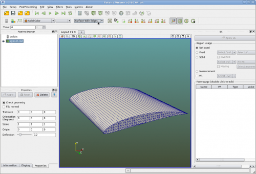
Run Polaris Viewer, import "sg6043.dat". Click and select "Surface with edges".
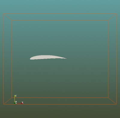
Next click on menu "Setup->Derived->Bounding Box", a bounding box of the airfoil is created. Change the name of the box to "simd" by double clicking "Box1" in the "Pipeline Browser". Then set X length and Y length to 25 and 20 respectively. Set the center of the "simd" box to (2.5, 0, 0.5). Click on "Apply" button in the "Properties" panel.
Next click on "sg6043.dat" in the "Pipeline Browser", and then click on menu "Setup->Derived->Bounding Box", another bounding box of the airfoil is created. Rename this bounding box to "vr". Set X and Y lengths to 3 and 2.4 respectively and center it at (0.8, 0., 0.5).
Click on "Save Project" and give a name of the project.
Setup the case
Definitions
Click on menu "Setup->Definitions". In the "Vectors and velocities" dialog click on vector "vx0" and set its magnitude to 60. This will be the incoming flow velocity. Hit "OK" to apply the change and close the dialog.
Click on menu "Setup->Case Setup". In the "Case Setup" dialog, there are multiple tabs. Set the following (accept all other default values):
| Tab Page | Parameter Name | Enter or Select Value |
|---|---|---|
| Global | Model dimension | 2D |
| Global | Analysis type | Turbulence k-e model |
| Global | Characteristic velocity | 60 |
| Global | Comments | tutorial to setup a 2d airfoil, Re=300,000 |
| Refinement | Simd length unit | meter |
| Refinement | Finest voxel size | 0.005 |
| Refinement | Finest level | 6 |
| Materials/Air | Kinematic viscosity | 0.0002 |
| Simulation domain | Bottom (-Y) | wall, frictionless |
| Simulation domain | Top (+Y) | wall, frictionless |
Click on the "Inlet/outlet" tab, then select "velo_in" to check the turbulence intensity. Use the default values if you do not wish to make a change.
Next click on "OK" to accept and close this dialog. The Reynolds number for this analysis is 300,000.
Save the project.
Assigning BC
Make sure that object "sg6043.dat" is highlighted in the "Pipeline Browser". In the BC panel, click "Solid" and then select "Regular Wall". Hit "Apply BC" on the top.
Click on "simd" in the "Pipeline Browser". In the BC panel, click on "Fluid" and then select the material "Air" and set the initial condition to "ic". Check "VR" and set it "0 coarsest". Click on "Apply BC".
Click on "vr" in the "Pipeline Browser". In the BC panel, check "VR" and set it "6 finest". Click on "Apply BC".
Save the project again.
Attack Angle
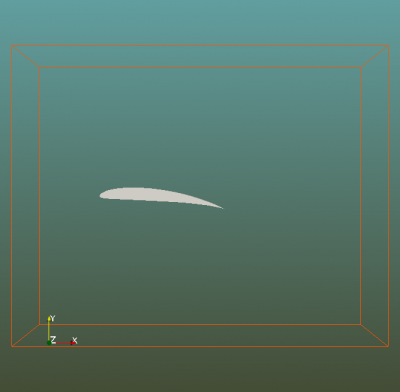
In Polaris CFD attack angle can be applied at the inlet by changing the velocity vector or at the airfoil by rotating the geometry. In this tutorial the attack angle is applied on the latter. Click on "sg6043.dat" in the "Pipeline Browser", in the "Properties" panel, enter -6 for the z component (third box from the left) of the "Orientation".
Job
Click on menu "Setup->Create a job". In the "Create/Edit Simulation" dialog, enter 0.2 for the "Courant number" and 10000 for "Total Steps". Then check these "Output variables": Fluid "Mach number", "Pressure coeff", Surface: "Pressure coeff". Click on "OK" to close this dialog.
Save the project.
Run the simulation
This simulation can be run on a desktop from a terminal or from the Polaris Viewer. It takes about 2 days using a desktop with 4 cores (i5, 3.0 GHz).
Analyzing the results
For airfoils, users are typically interested in the lift and drag. Open the force output file in Polaris Viewer or in a text editor, one can find the drag Fx=79.5 N/m, lift Fy=2881.1 N/m, the air density=1.293 kg/m^3 as reported by the solver, the characteristic velocity=60m/s, characteristic length=1m, one can compute Cd=0.034, Cl=1.235 which match the results in Summary of Low-Speed Airfoil Data.
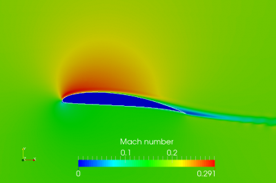
In Polaris Viewer, load surface result file and set the view mode to "Wireframe". Load the fluid result file and set the view mode to "Surface" and then pick "Mach number" as the display variable. Go to the last timestep. Zoom in to the airfoil and one can observe this plot.
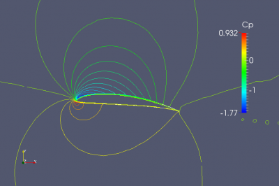
One can plot isolines for 2d fluid results. First click on the fluid file in the "Pipeline Browser", then click on menu "Filters->Alphabetical->CellDataToPointData". Hit "Apply" in the "Properties" panel to convert fluid cell data to point data. Then click on the "Contour" button in the toolbar or in the "Filters" menu. Select "Cp" as the "Contour By" variable. Click on "New Range" in the "Properties" panel and set 21 intervals. Hit "Apply" in the "Properties" panel to see the isolines. The isolines initially are white. Users can color them by a variable.
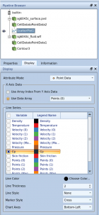
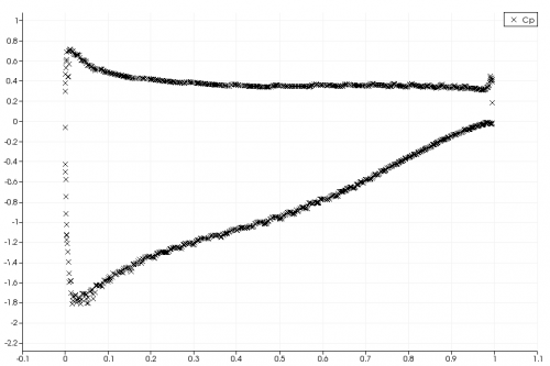
To plot the Cp against chord position, first click on the surface result file in the "Pipeline Browser". Then click on menu "Filters->Alphabetical->CellDataToPointData". Hit "Apply" in the "Properties" panel to convert surface cell data to point data. Then click on menu "Filters->Alphabetical->ScatterPlot". Hit "Apply" in the "Properties" panel to convert surface cell data to point data. An x-y chart is shown in the main view. Activate the "Display" panel, set "X Axis Data" to "Use Data Array->Points (0)". In the "Line Series", uncheck all except "Cp". Click on "Cp" there and set "Line Style" to "None" and "Marker Style" to "Cross".
